Codecs and Compression
When I say PCM, ADPCM, or GSM, do you do you have any idea what that means? There seems to be a bit of confusion among those working with digital telephony about what codecs are. I'm going to address some of the basic concepts. First, understand that the major goal is to compress a signal (usually speech or music) to the highest possible degree at the maximum possible quality. The larger the compression ratio is, the lower the quality tends to be. And good compression often means lots of computation.
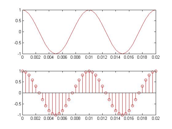
Let's start with the basics. What happens when you talk into a microphone? There is a spherical pressure wave. The microphone transduces the wave into an analog electrical signal. But we need the signal stored digitally in a computer if we're really going to do something useful to it. So the next step is to sample with an analog to digital converter (ADC). All this can be done with a cheap microphone and sound card. In the figure below, .02 seconds of a pure tone has been sampled. Once this happens, you lose information that was stored in the analog waveform. But that's ok. If done correctly, it's safe to throw away information. Also notice that the samples are uniformly sampled in time. The inverse of the time between the samples is the sampling frequency. At this point, if nothing else were done to the sampled signal except storing it on disk, we would call this Pulse Code Modulation (PCM). That's all an uncompressed wav file is - some header information followed buy a list of numbers. Each number is a sample. The larger the number is, the stronger the pressure wave and voltage signal was at sample time. Wav files can also store other codecs as well. That information would be in the header.
I said we can throw away information. The closer together the samples are, the more frequencies are represented in a signal. As an example, the human hearing range is about 20-20000hz. If the sample rate is 40khz, the time between samples is 25 micro seconds (the inverse thing), and all of the human hearing range has been safely stored. This is known as the Nyquist rate. The sample rate has to be more than twice the maximum frequency you want to keep. Have you ever seen 44.1khz? Half of this is just above the human hearing range. A lower quality signal, such as one used by the telephone companies, is had by sampling at 8khz. The phone companies actually filter the analog signal at about 3300hz. This allows just enough frequency information through to recognize someone's voice and understand what they're saying. Although you could sample this signal at a much higher rate, there isn't any reason to because the high frequency content has already been removed. And you want to get the sample rate as low as possible. A high sample rate means a more expensive ADC and more samples to store and process.
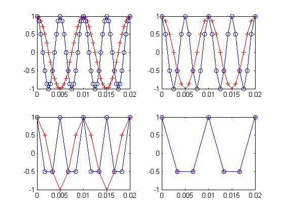
When the signal is sampled, the frequencies that are greater than half the sample rate have to be removed or they cause what's known as aliasing. Take a look at the plots below. In the upper left plot, there are two signals. One is blue with samples occurring at the circles. The other is red with samples at the plus signs. The blue wave is at 200hz, the red at 100hz. The sample rate is 2400hz. Move to the right. The sample rate is now 1200hz. Looks good, right? Now move to the bottom left. The rate is 600hz. It's starting to look ugly, but that's ok. We're still safe at this sample rate. In the final frame, at 300hz, we see the signals exactly overlap. What happened? Well, 300hz isn't more than twice 200hz (the blue one). It aliased and moved down 100hz so that it exactly lies on top of the 100hz signal. Notice in the previous frame there were about three samples per sinusoidal cycle. In the last frame there are less than two samples per cycle. How can you know the difference between a lower frequency and a higher one if there are so few samples? You can't. And in this case the samples for these two waves exactly overlap; so they appear to be the same. Solving this problem requires an anti-aliasing filter. The higher frequencies have to be removed before sampling (or they can be removed after, but the sample rate would have to be much higher than what we intend to use). In any case, the information we don't want is removed, and you're left with only the frequency content that lies at less than half the sample rate.
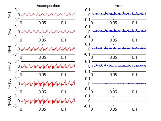
For the remainder of this explanation, you'll need to have the appropriate images in your head to adequately understand what I'm saying. Have you ever looked at a plot of a speech waveform? It probably looked mostly meaningless to you. Fortunately, there is an easier way to understand complicated looking waveforms. You can think of it as a summation of sinusoids. In the plots below, a segment of speech has been decomposed into sinusoids. This is actually one way to do compression. You could just throw away the less important sinusoids - ones with small amplitudes. The left column shows the sinusoids being added back together. For the case of N is one, only the largest sinusoid is taken. When N is two, the two largest sinusoids are added. If you add all the sinusoids together you get back the original signal. The right column shows the error between the original signal and the partially decomposed signal. Don't worry about how to decompose the signal, just remember, whenever you do something to a signal, you can do it to just the sinusoids and then add them together. It's much easier to think about what's going on in this manner. A sinusoid is very simple. There are only three things you can do to it - (1) Change the amplitude (stretch vertically), (2) change the frequency (increase horizontal distance between maximums), and (3) change the phase (where it starts). And often for speech signals, the phase isn't all that important. So you can mostly just think about scaling and stretching a very simple looking waveform. Another picture you should have in your head is an empty plot of the power spectrum (or frequency domain). Any time I say frequency, you should be seeing power on the vertical axis and frequency on the horizontal axis. A sinusoid (or pure tone) in the time domain is going to look roughly like a vertical line in the power spectrum. The height corresponds to power. The position on the horizontal axis is the frequency of the sinusoid. If you add two sinusoids of different frequencies together, you'll get two peaks or lines.
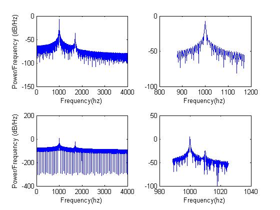
If you were going to compress a bunch of numbers, how might you start? Throw the least important information away. One easy way to do this is to set the sample rate as low as possible, so you have less numbers in the first place. Another thing you might try is psychoacoustics. When two different frequencies of equal power (same height sinusoids) are close together you get what's called beating. However, if one has much more power than the other, the lower power tone is harder to hear. As a demonstration, the plots below show three frequencies - 1000hz, 1010hz, and 1700hz, with the last two at lower power. The top left plot shows the power spectrum. The top right shows the same thing on a smaller frequency scale. Notice how you can't see 1010hz? This is actually the result of taking frequency transforms with too few data points. The resolution isn't good enough. The bottom plots are exactly the same, but the time domain signals had a longer duration. You should be able to make out 1010hz. The brain, similarly, cannot hear certain frequencies when they are occasionally masked by other more powerful ones. MP3s use this fact to throw away more information when that information can't be heard. Listen to the tones displayed below and to the same tones with equal power. In both cases the first third is 1000hz, the second third is 1000+1010hz, and the last third is 1000+1700hz. Another trick is shaping noise in the frequency domain. Your brain can't hear noise at about -13dB relative to a pure tone in the same frequency range. You could move the noise around so that it rests around the frequency content you want to hear and that will act as a noise mask.
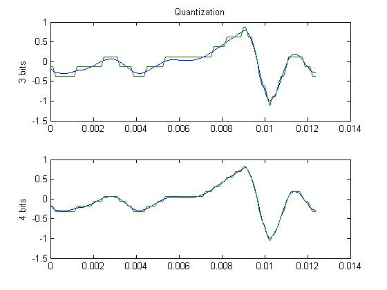
A more common way to throw away information is by quantizing differently. You saw earlier that the waveform was discretized at regular intervals. This produced a list of numbers representing the signal. However, we also have to consider the size of those numbers. If the numbers are allowed to be very large (say 16 bits), each sample will be very close to the original value of the pre-sampled waveform. If the numbers are only a few bits in size, the error will be large. You can think of this as adding noise to the signal. The plot below shows a waveform sampled at three and four bits. So you could double your compression by reducing from 16 to 8 bits with a loss of quality. Note that no frequency information is lost. It's just that there is more noise in your signal. That's important. More samples (numbers) means more frequencies. Larger range (bigger numbers allowed) means less noise.
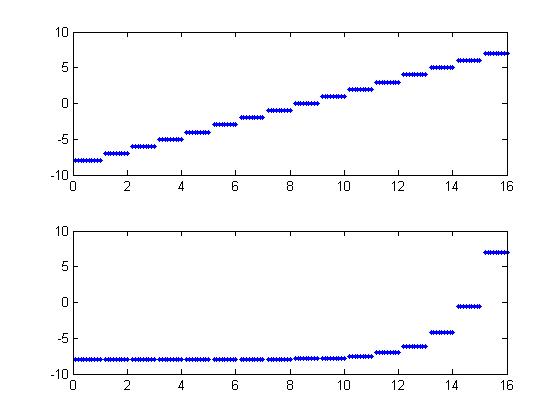
Ok, so how do we get better compression without sacrificing too much quality? Well, the simplest technique used for speech is to quantize non-linearly. Speech tends to have a lot of low power information but a large dynamic range as well. By quantizing on a logarithmic scale, you can get the large numbers without sacrificing the accuracy of the small numbers. The plot below shows how logarithmic quantization might work. The horizontal axis is the old value, and the vertical access is the quantized value. The top plot shows a linear quantization and the bottom one a logarithmic quantization. This is essentially how ulaw and alaw work. The difference between them is just a slightly different logarithmic mapping. With fewer bits you can get a speech signals with the same amount of noise.
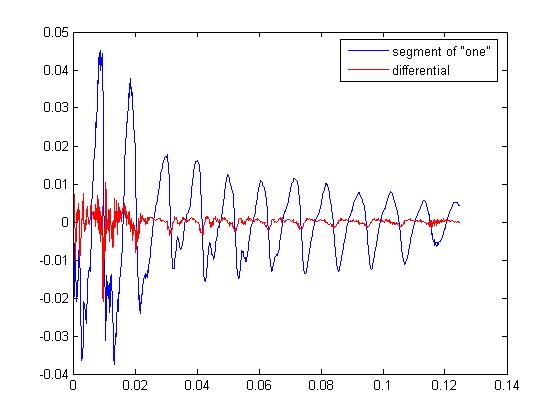
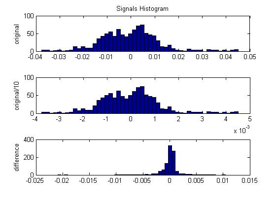
Another method of reducing the number of bits is decorrelation. A highly self correlated signal has a lot of redundant information in it. Applying a process to decorrelate, or remove redundant information, or reduce the variance or power allows the signal to be represented with fewer bits. Differential Pulse Code Modulation (DPCM) is one of the simpler ways of doing this. At every sample, you want to try and predict that sample and then subtract the prediction from the sample. If your predictions are good, your new numbers will cover a smaller range and you can use less bits to represent the new signal. How do you make predictions? First, the predictions have to be based off the signal itself so that we can reverse the process during decompression. Second, since we're assuming the signal is self correlated, we can use the previous n samples to predict the current sample. In the simplest case, just subtract the last sample from the current sample. An easy way to understand why this works is to think of a line. After applying this process to the line, you're left with a constant at the slope of the line. How many bits does it take to represent this signal (assuming a very long duration)? Almost none! You can just record the slope of the line and the duration and that's it. A more realistic example is shown in the plot below. This is an actual portion of speech. The blue signal is the original. The red one is the difference. You could do even better using prediction with more samples. An improvement on DPCM is Adaptive DPCM (ADPCM). ADPCM adapts the quantization scale based on the size of previous samples. If the last sample was small, the next sample will probably be small (correlation again). So why not make the quantization range smaller? Because you don't have to choose a fixed quantization scaling that has too few bits at low power and too many at high power, the number of bits can again be reduced for a given quality signal. Before I continue, I just want to make sure you understand that scaling doesn't just change every sample in the same way. You actually have to modify the signal statistics in some significant way. Look at the 'Signals Histogram' figure. The top plot (of 3) is a histogram of the signal. The one below it shows the histogram of the same signal but the magnitude has been divided by ten. Notice how the histogram didn't change. The last one is with DPCM applied. The shape of the histogram is different. It looks like more of the samples are hanging around zero.
I'll briefly mention a few more compression methods. One is vector quantization. The idea here is to quantize several samples at once instead of each one individually. Because of that correlation thing again, a group or vector of closely clustered samples tend to have similar values. You can use this information to decrease the range the vectors cover or throw some of them out, thus reducing bits. A really high rate of compression can be had through Linear Predictive Coding (LPC). The idea is to use linear prediction to build a prediction filter out of a small number of coefficients. The statistics of speech don't change very much over short durations. This lets you reduce the entire frame of speech to a small filter and fundamental frequency that can predict the entire frame. Another way of thinking about this is that you're building a model of the vocal tract. You can extract only the parameters that you need, such as the fundamental frequency the voice box produces, and the complex envelope (or formants) created by your mouth and tongue. These formants (equivalent to the prediction filter) are the resonances that determine what sound you make. Once you extract these parameters, you can throw the rest of the information away. At decompression, you can use the parameters along with your model of the vocal tract to recreate the signal. Although you can get very good compressiont his way, the quality is not very high since you've thrown so much information away. But as long as you have the first few formants, it's still intelligible speech.
Most codecs are some variation on the above mentioned techniques. There are likely hundreds of minor variations. Anything you can think of that will strip out information you don't need can be used to reduce the number of bits per sample. There is usually a trade-off among quality, amount of compression, and time of compression/decompression. A very low bit rate usually means much lower quality and probably good amount of computation. Consider an extreme case. What if I had a program that could perfectly model my entire vocal tract? On one end, I could use speech recognition to record my speech as text. I could send compressed text at an extremely low bit rate and have it reproduced on the other end at high quality sounding exactly like me. There are a few problems with this of course. One is the amount of computing power you would need to model my entire vocal tract and probably parts of my brain. The other is that the speech still won't be the same. It doesn't consider things like volume, speed, and my emotional state at every instant. However it does demonstrate, at least in principle, that a very high quality, low bit rate codec could be built if you had enough computation power.
Matlab scripts:
decomp.m
demo_codecs.m